

If you are not familiar with Google Kaggle, I recommend you read my previous article for a high-level overview of what you can expect from this platform. TLDR: It is a portal that allows users to create artificial intelligence centred challenges (paid and non-profit ones). The users can participate in challenges and share their solutions via special notebooks which can be viewed and commented on by the other users. In this article I will guide you through a legendary Titanic Challenge! It is considered the best way to start your journey with Kaggle. So, if you are planning to participate, please do read the solution part of this article. Maybe, come back to it when you run out of ideas within your own notebook. The challenge can be found here.
In this article I will share the implementation details of a data processing pipeline, the goal of which is to transform a raw dataset provided by Kaggle into usable machine learning training data.
It is a numbers game!
In the part 1 of this article we have introduced a high-level “run_complete_pipeline_transformations” method. We will now go into each of the sub-method implementation details to learn how we go from zero to hero with our Kaggle dataset.
Let us start from the top with the general pre-processing sub-method. Each line is a different transform that we will run on our input Pandas DataFrame. The first step is some general pre-processing (the explanation will follow the code):
@staticmethod
def transform_csv_preprocessing(data):
    data['Sex'] = data['Sex'].map({'male': 0, 'female': 1})
    data['Embarked'] = data['Embarked'].map({'S': 0, 'C': 1, 'Q': 2})
    data['FamilySize'] = data['SibSp'] + data['Parch'] + 1
    data['IsAlone'] = 0
    data.loc[data['FamilySize'] == 1, 'IsAlone'] = 1
    data['NameLength'] = data['Name'].str.len()
Neural networks do not work well with strings. I have mentioned before that their job is to find a function of x that accurately calculates the value of y. With this in mind we cannot multiply or concatenate strings… Well, we could I guess if we tried really hard but for this scenario let’s assume that we cannot and should not. What we will do is we will map the ‘male’ strings to a numeric 0 and ‘female’ to 1.
Another thing we can do is to create new columns that may help the network in training. You have to think about the network as an extremely good pattern finder, you need to provide it with as much clear information you can for it to find the right patterns. In this case we can hypothesize that a size of passenger’s family may have some influence on his/her survivability. To test this hypothesis, we will create a completely new column ‘FamiliSize’ which will be computed as a concatenation of ‘Parch’ and ‘SibSp’ columns. In a similar way we will create a binary column ‘IsAlone’. Perhaps our new columns will influence our pattern finder, perhaps not. We need to test it anyway as we are data scientists and this is what we do. One last column I came up with is the ‘NameLength’ column – I figured aristocrats and rich people in general often had these long names combined with titles like that German guy Hubert Blaine Wolfeschlegelsteinhausenbergerdorff Sr. Maybe there is something here, maybe not, we will see.
Next thing we will be looking at is each individual’s Title as written on their ticket (Dr/Sir/Miss/Major etc.). Analysing the data can be done with Pandas Crosstab:
pd.crosstab(data['Title'], data['Sex'])
We can see the count of every title in the dataset across men and women:
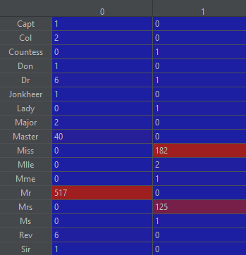
We can see that the couple of values represent a majority of dataset, so it makes sense to remove the other values to avoid negative impact on our network training. It would however be a bit wasteful to just remove these rows especially with a dataset this small. What we can do instead is put them all to a new aggregator category so that the Title can still be usable:
@staticmethod
def transform_csv_create_title(data):
    data['Title'] = data.Name.str.extract(' ([A-Za-z]+)\.', expand=False)
    data['Title'] = data['Title'].replace(['Lady', 'Countess', 'Capt', 'Col', \
                                                 'Don', 'Dr', 'Major', 'Rev', 'Sir', 'Jonkheer', 'Dona'], 'Rare')
    data['Title'] = data['Title'].replace('Mlle', 'Miss')
    data['Title'] = data['Title'].replace('Ms', 'Miss')
    data['Title'] = data['Title'].replace('Mme', 'Mrs')
    title_mapping = {"Mr": 1, "Miss": 2, "Mrs": 3, "Master": 4, "Rare": 5}
    data['Title'] = data['Title'].map(title_mapping)
    data['Title'] = data['Title'].fillna(0)
Bucketizing
Next, let’s go over a useful technique call bucketizing, it allows us to divide a series of data into labelled ranges/groups. We could for example replace the age column with the age band representing young, old and middle age people. Because the training is on a high-level multiplication of numerical feature values by initially random network weights – this 3 categories/values feature will have a better impact on our training than a feature with 80+ possible values. We can create a new column representing age groups as this:
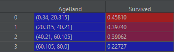
data['AgeBand'] = pd.cut(data['Age'], 4)
In here we will create 4 equally spread age groups. Given below is the visualization of each group’s survivability:
data[['AgeBand', Survived]].groupby(['AgeBand'], as_index=False).mean()
Of course, you are not limited to equally spread bands, you can decide the age ranges after analysing the data a bit further. Here is how you can do that on example of widely spread columns “Fare” and “Age”:
data['Fare'] = pd.cut(data['Fare'], [0,7.911,14.455,31.01,90000]).cat.codes
data['Age'] = pd.cut(data['Age'], [0, 10, 18, 26, 36, 50, 65, 200]).cat.codes
Filling out the blanks
We will now use two techniques for filling NaNs – missing values. First, it is fairly obvious and we will demonstrate it on the “Embarked” column.
As you can see with a command summing all the missing values in our dataset:
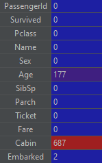
There are only 2 rows missing this value but it is still worth filling it if we can – and we can with the use of .fillna() method which we will use passing it to the most frequent part from the dataset. We are guessing here but an educated guess should still be better than no value at all in a lot of cases. The second scenario will be a slightly more complicated guess. We will fill the missing age values based on the most-often occurring age for our “Title” and “Class”. Hopefully, the code will explain itself here but if it does not, the explanation is as given below:
@staticmethod
def transform_csv_generate_missing_age(data):
    for index, row in data.iterrows():
        if math.isnan(row['Age']):
            curr_title = data.at[index, 'Title']
            curr_pclass = data.at[index, 'Pclass']
            maching_group = data.loc[
                (data["Title"] == curr_title) & (data["Pclass"] == curr_pclass), "Age"]
            mean_age = maching_group.mean()
            std_age = maching_group.std()
            normal_guess = np.random.normal(mean_age, std_age)
            data.at[index, 'Age'] = normal_guess
    data['Age'] = data['Age'].astype(int)
We are iterating over all the rows with the missing age values, and for each row we locate a subset of rows from our dataset matching our Title and Class. From this sub-group we could just take an average value but this would leave us with a lot of values with exactly the same value, and this could create an artificial pattern that would affect our network training. What we will do instead is a pretty standard way of getting more naturally random value centred on the average for a particular group. The way to do it is to calculate the mean value and then the standard deviation describing how far from the mean values usually are. Based on these two values we can create a random value with a specially prepared helper method from numpy library.
Honey, I Shrunk the Values!
For many reasons, it is important that the feature values are in a similar numerical range or scale. If we had few features with values ranging from 0 to 2 and a single feature with values coming up to 100 or higher, the higher value feature column would mathematically overshadow the smaller ones. When I say overshadow, I mean making them statistically less relevant than they possibly really are. Second thing that could happen is what’s called overfitting – it’s basically destabilisation of your training process due to extremely high model weights that can cause numerical overflows and create a lot of NaN weights in your model, eventually crushing the training loop. The training is mostly multiplication and we cannot multiply by “Not aNumber”). The way we can approach this could not be simpler in Python. All we need is a helper class of the very useful SkLearn toolkit called the MinMaxScaler.
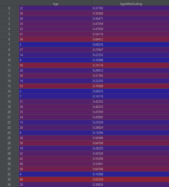
@staticmethod
def transform_csv_scale_to_one(data):
    scaler = MinMaxScaler()
    data['NameLength'] = scaler.fit_transform(data[['NameLength']])
    data['Pclass'] = scaler.fit_transform(data[['Pclass']])
    data['Fare'] = scaler.fit_transform(data[['Fare']])
    data['Age'] = scaler.fit_transform(data[['Age']])
    data['Title'] = scaler.fit_transform(data[['Title']])
    data['Embarked'] = scaler.fit_transform(data[['Embarked']])
As you can see we are not even passing any parameters to our scaler as by default it is configured to scale from 0 to 1. The output of this transformation on our “Age” column would look like this:
Final clearance
The last thing to do is to remove all the columns that we have no use for as they contain no statistical relevance, or we have already extracted the useful information out of them to the other columns.
@staticmethod
def transform_csv_postprocess(data):
    return data.drop(['FamilySize','SibSp','Parch','Name','Ticket','Cabin','PassengerId'], axis=1)
The aforementioned code gives us a dataset that better suit for any mathematical operations attempting to find the relationship between the feature columns and label column “class”.
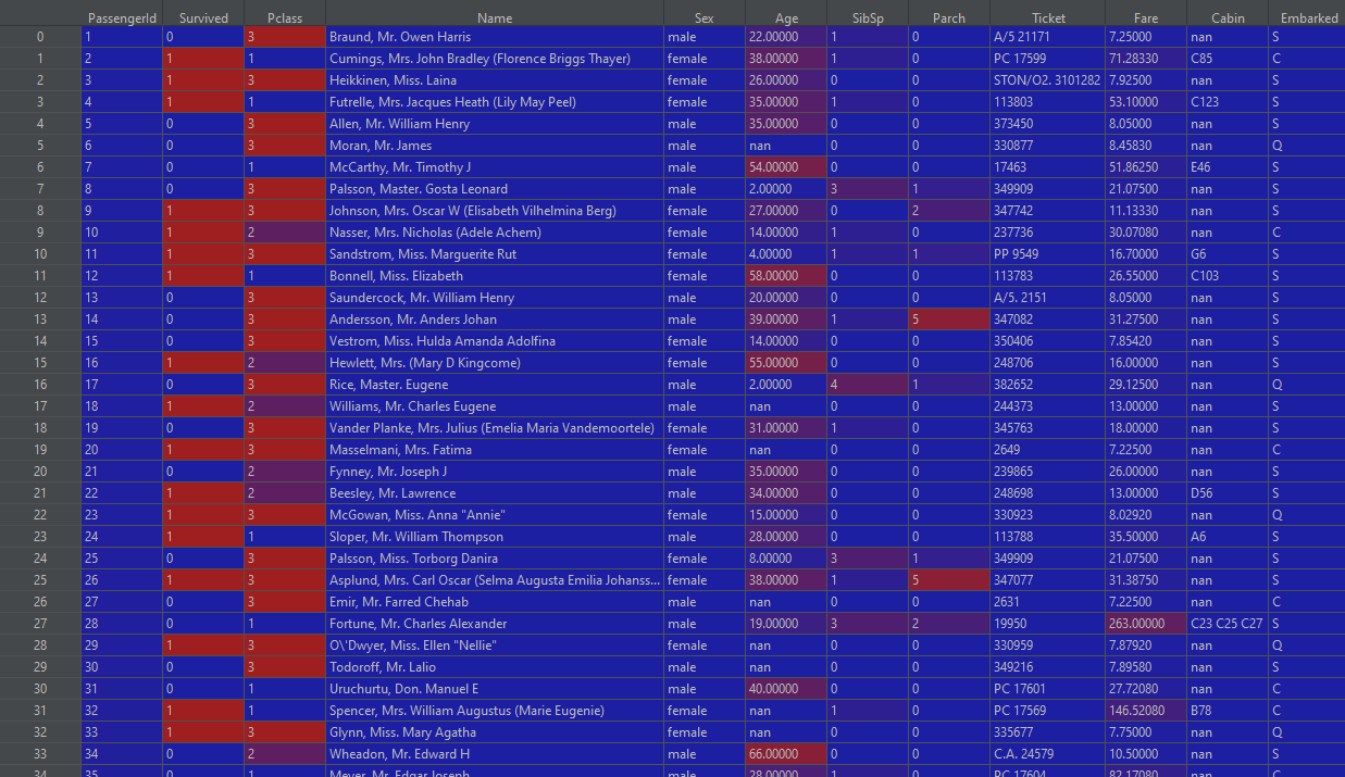
Before:
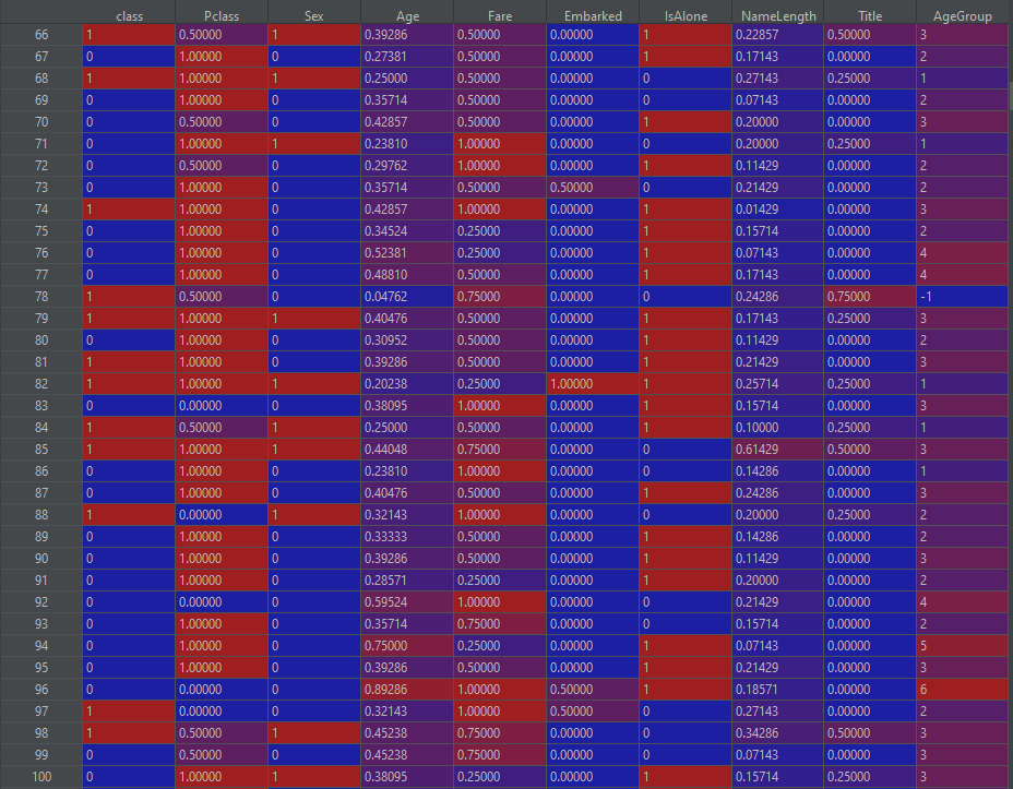
After:
This concludes our data processing pipeline. The data should now be a perfect fit for neural network training which you can see in my github here. The key aspect that we have to look at are test1_dnn.py which is a file containing the model and training code for the above pipeline and the KaggleHelper.ConvertProbabilititsToClasses method which converts network output predictions to the format expected by the Kaggle submission.
Author of this blog is Patryk Borowa, Aspire Systems.